Thermal Imaging

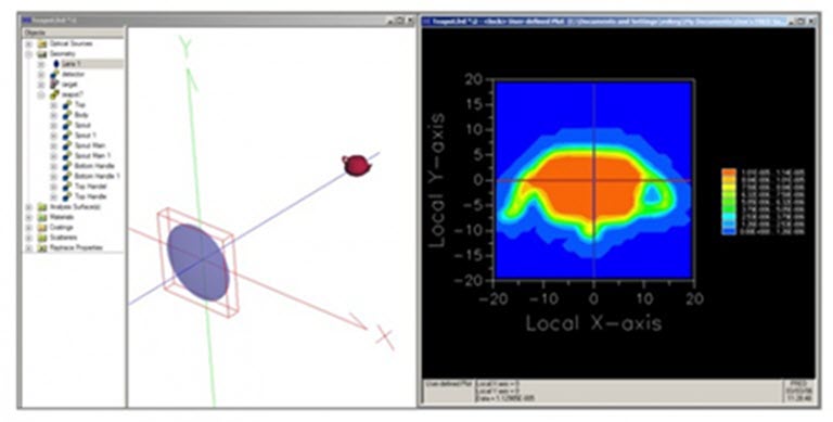
Thermal imaging is a key technology for defense and detection applications such as the classification and tracking of concealed weapons, personnel, vehicles, and objects. Recently, efforts have been aimed at expanding IR sensing to temperature measurement and mapping, forest fire sensing and suppression, surveillance, and multi-spectral earth imaging.  Figure 1 shows an example of simple thermal imaging model in FRED: a teapot is imaged through a camera lens by an infrared detector. 

Figure 1. A warm teapot with different emissivities and temperature distribution across its surface is imaged through a singlet into a detector.

A key challenge in thermal imaging is noise. To combat this, systems typically subtract nominal background radiation to enhance contrast in the infrared scene. If the background is not uniform, however, a stray signal can be produced. Two sources that cause this variation are thermal emission and narcissus. Thermal emission is energy emitted from the environment or optical instrument that causes an increased signal in the detector.  Narcissus, on the other hand, is a ghost image produced by a cooled detector array which reflects off of lens surfaces and re-enters the detector as a reduced signal: a dark, circular region. 

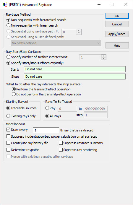
FRED has the capability to do an advanced raytrace that keeps track of all ray paths in a system. This is accomplished by selecting [Raytrace > Advanced Raytrace…] from the main menu and checking “create/use ray history” and “determine raypaths” options (Figure 2). 

Figure 2. Advanced Raytrace dialogue with create/use ray history file option and determine ray path options checked.

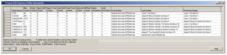
After performing a raytrace, select [Tools > Reports…. Raytrace Paths…] from the main menu to produce report detailing how each ray paths reaches each surface (Figure 3). By using this method, it is possible to see how much power each of the ghosting, straight shot, single or multiple scatter paths contribute compared to the signal path.

Figure 3. Ray Paths for the Teapot Example shown in Figure 1. Path #1 is the direct thermal contribution from the teapot.

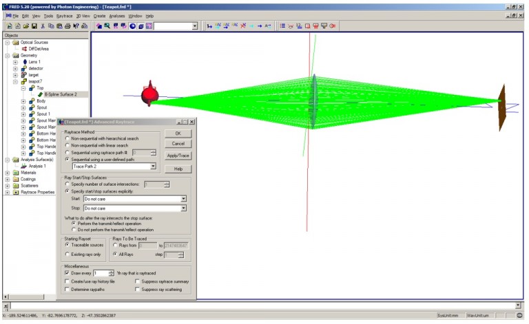
It is also possible to take a specific ray trace path and copy it to a user defined path list. Simply select the path, right mouse click and select the option to copy it to the user-defined path list. This path will now show up one of the ray methods to use in the advanced raytrace (Figure 4). Using this capability, spot diagrams and irradiance spread functions can be created for a single path.

Figure 4. Path #2 from the ray path report in Figure 3 is selected for an advanced raytrace. The raytrace of this path is shown for the teapot example. 

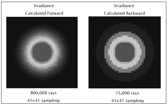
There are several methods to simulate thermal emission in FRED. One technique is to create a source and raytrace it though the optical system. Another approach is to raytrace backwards from the detector through the system. Reverse ray tracing requires fewer rays, and is therefore a much more efficient. Faster ray tracing can allow one to assess the effect of incremental changes on the design in “real time”.  A comparison of forward and reverse ray tracing detector images is shown in Figure 5:

Figure 5. Comparison of two irradiance calculations: one performed using forward ray tracing and the other using backward ray tracing.  The latter required 53x fewer rays to reach the same level of accuracy.

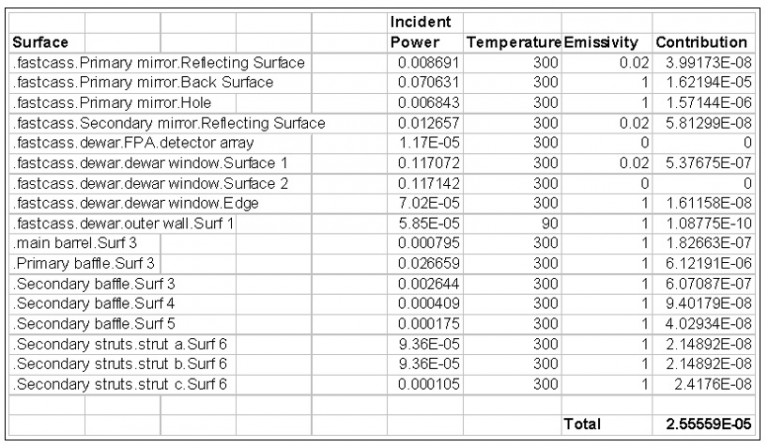
Thermal self-emission is the radiation of energy from structures within the system. If this energy is collected by the detector, it will contribute to a stray light signal.  Each object in the system radiates as a function of temperature and emissivity. One way to quantify self-emission is to model each contributing surface as a Lambertian light source with appropriate energy and spectrum. However, this approach is incredibly inefficient! The detector fills a very small solid angle relative to the emission angle of these sources. A better approach is to perform a reverse raytrace from the detector and apply some radiometric concepts. The equation for thermal self-emission of a system is given by:

where ε = emissivity, f = fractional blackbody integral, σ = Stefan-Boltzmann constant, T = temperature (deg K), Adetector is detector area and (Ωobject/π) is projected solid angle of an object with respect to the detector.  

It can be shown that power received by each object is numerically equal to its projected solid angle ¹. Therefore, to determine TSE, one can perform a reverse raytrace in FRED. After the raytrace is complete, incident power on each object can be obtained. This value may be substituted for (Ω/π) in equation 1. TSE contribution from each object can be calculated, given values of T and ε (Figure 6).

Figure 6. Calculating thermal self-emission from a Cassegrain telescope using a spreadsheet such as Excel. The column “Incident Power” is actually projected solid angle of the object. The column “Contribution” implements eq. 5.

Using advanced raytracing capabilities in FRED, along with techniques derived from radiometry, it is possible to perform thermal imaging, narcissus, stray light, thermal illumination uniformity, and thermal self-emission calculations in a small fraction of the time it would take to trace the requisite number of rays in a brute force manner. FRED can also track each path traced through the system. The Raytrace Paths Report provides the contribution of each path to power reaching the detector. With these tools, one can quantify the effect of spurious signals in the detector and add features to the system to reduce these effects.

¹R. Pfisterer, “Clever Tricks in Optical Engineering” (invited paper), Proceedings SPIE, Vol. 5524, October 2004.