Stepping a Raytrace for Analyses

Introduction

Analysis Surfaces in FRED post-process (filter) rays at the end of the raytrace when an analysis is requested. They do not collect ray information during the raytrace, even when the ray trajectory passed through the analysis grid on it's way to it's final location.

So in these situations, how do we analyze the optical field in an optical space for rays passing through that space during the raytrace?

One option can be to use FRED’s Detector Entity constructs. Detector Entities are similar to Analysis Surfaces except that they can be inserted into any optical space and can collect ray information dynamically during the raytrace (i.e. as rays pass through the collection grid). However, Detector Entities do not currently work with coherent or polarized rays and can only perform Irradiance, Illuminance and Color Image analyses.

The purpose of this article is to demonstrate how we can setup our system in such a way that a simple script can be used to access ray information at any position during the raytrace using Analysis Surfaces.

Setting up the Calculation

Download the FRED file: steppedARTwithAnalysisExample.frd

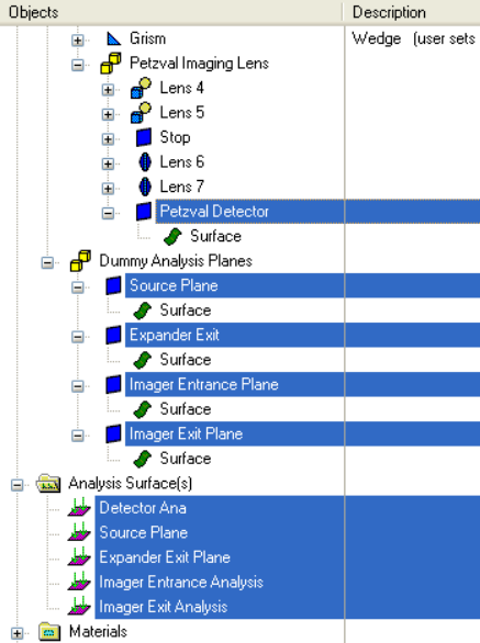
This article uses the optical system shown in the image below. Our intention is to analyze the irradiance distribution of a coherent source at various planes in the optical path.

We will perform this operation by inserting several optically transparent dummy plane surfaces at the desired locations and then attach standard analysis surfaces to each dummy plane. When we perform the analysis, we will use the Advanced Raytrace feature to step the rays from one plane to the other and perform the irradiance calculation at each plane within an embedded script.

Breaking the trace into several pieces is the central "trick" to being able to use analysis surfaces to generate data during the trace.

The image below shows the plane surface geometry and analysis surfaces that are used in the manner described above.

Performing the Calculation

Within the document is an embedded script calculation called “SteppedAdvancedRaytraceAnalysis” which can be run by simply right mouse clicking on the embedded script and choosing to run it. Information will be reported to the output window regarding the status of the script execution. After the script has completed, the irradiance distributions at each plane of interest will be displayed in context in the 3D view. :

Optionally, the user can right mouse click on the ARNs and choose to display each in the chart for additional detail.

Explanation of the Scripted Calculation

The raytrace and analysis has been automated in an embedded script in the document called “SteppedAdvancedRaytraceAnalysis”. The first section of the script is a generic “Document Cleanup” section in which we prepare the document and output window for the analysis that will be performed.

The next section of code defines two array variables, anaPlanes() and anaSurfs(), which contain node number references to both the dummy plane geometry (where we’re stepping the rays to in the raytrace) and their corresponding analysis surfaces. In this example, there are 5 planes along the optical path at which we want to analyze the beam.

Next, we prepare the advanced raytrace so that we are tracing rays that currently exist in the buffer (not tracing from the sources directly). This allows us to pick up our current rayset where we left off and then propagate it to the next plane of interest. Additionally, we create the starting rayset from the sources directly.

Once we’ve entered our FOR loop, which is the core of the raytrace/analysis routine, we first step the rays to the current plane of interest. The FOR loop counter serves to identify the current plane of interest by using it as an index into the two arrays we defined previously. We set the current surface we wish to stop on in the T_ADVANCEDRAYTRACE structure variable and call the AdvancedRaytrace.

Now that we are at the current plane of interest, we perform the irradiance calculation at the current plane and store the result in an Analysis Result Node (ARN).

Now that we have the analysis result at the current plane, we can perform a statistical analysis on that result and report information to the output window.

At this point, we have exited the FOR loop and have all of the ARNs on the object tree containing the results of our analyses. The last step is to loop over all of the ARNs and display them in the visualization view.